

Step-by-step guide on using theDuring this walkthrough, we will become familiar with the mainAutoTheta ModelwithStatsforecast.
StatsForecast class and some relevant methods such as
StatsForecast.plot, StatsForecast.forecast and
StatsForecast.cross_validation in other.
The text in this article is copied from and inspired by: 1. Jose A.
Fiorucci, Tiago R. Pellegrini, Francisco Louzada, Fotios Petropoulos,
Anne B. Koehler (2016). “Models for optimising the theta method and
their relationship to state space models”. International Journal of
Forecasting.
2. Rob J. Hyndman and George Athanasopoulos (2018). “Forecasting
Principles and Practice (3rd ed)”
Table of Contents
- Introduction
- Loading libraries and data
- Explore data with the plot method
- Split the data into training and testing
- Implementation of AutoTheta with StatsForecast
- Cross-validation
- Model evaluation
- References
Introduction
TheAutoTheta model in StatsForecast automatically selects the best
Theta model based on the mean squared error (MSE). In this
section, we will discuss each of the models that AutoTheta considers
and then explain how it selects the best one.
1. Standard Theta Model (STM)
The Standard Theta Model is the original version of the Theta model introduced by Assimakopoulos and Nikolopoulos (2000). It decomposes a time series into two modified versions of the original series, called theta lines. These lines are created by applying a linear transformation to the second differences of the original series, controlled by a parameter called theta . One theta line captures the long-term trend, while the other captures short-term fluctuations. The two theta lines are then combined to produce the final forecast. The STM assumes that model parameters remain constant over time.2. Optimized Theta Model (OTM)
The Optimized Theta Model extends STM by searching for the best theta parameters rather than using fixed values. This optimization step allows the model to better fit series with higher variability.3. Dynamic Standard Theta Model (DSTM)
The Dynamic Standard Theta Model allows STM to adapt over time. Instead of keeping parameters static, it updates them dynamically as new data becomes available. This dynamic behavior can be useful when forecasting series with evolving trends or seasonality.4. Dynamic Optimized Theta Model (DOTM)
The Dynamic Optimized Theta Model combines features of both OTM and DSTM. Like OTM, it optimizes the theta parameters. Like DSTM, it updates the model dynamically with new data.How AutoTheta Selects the Best Model
AutoThetafits all four variants of the Theta model (STM, OTM, DSTM, and DOTM) to your data.- Each model is evaluated using cross-validation or a hold-out validation strategy, depending on the configuration.
- The model that achieves the lowest mean squared error (MSE) is selected.
- The selected model is then used to generate the forecast.
Loading libraries and data
Tip Statsforecast will be needed. To install, see instructions.Next, we import plotting libraries and configure the plotting style.
Read Data
The input to StatsForecast is always a data frame in long format with
three columns: unique_id, ds and y:
-
The
unique_id(string, int or category) represents an identifier for the series. -
The
ds(datestamp) column should be of a format expected by Pandas, ideally YYYY-MM-DD for a date or YYYY-MM-DD HH:MM:SS for a timestamp. -
The
y(numeric) represents the measurement we wish to forecast.
(ds) is in an object format, we need
to convert to a date format
Explore Data with the plot method
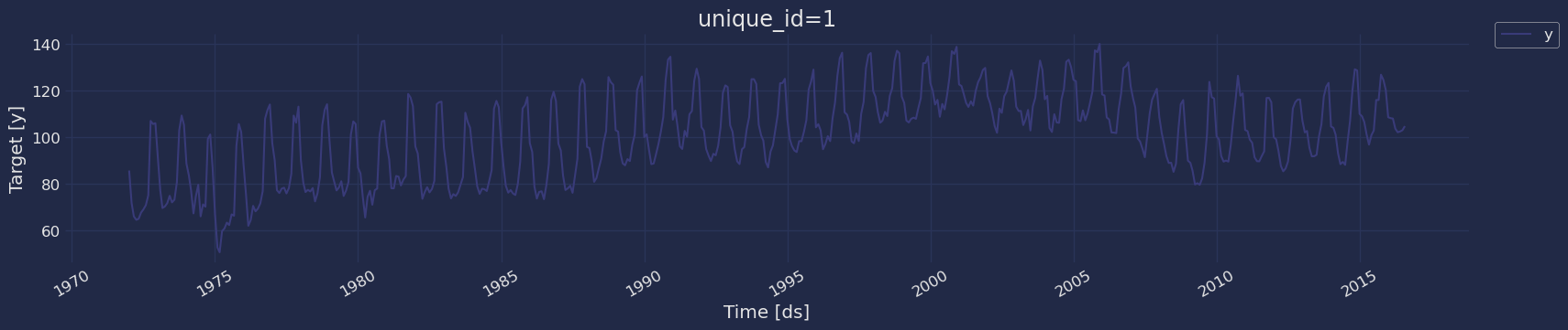
Plot some series using the plot method from the StatsForecast class. This method prints aa random series from the dataset and is useful for basic EDA.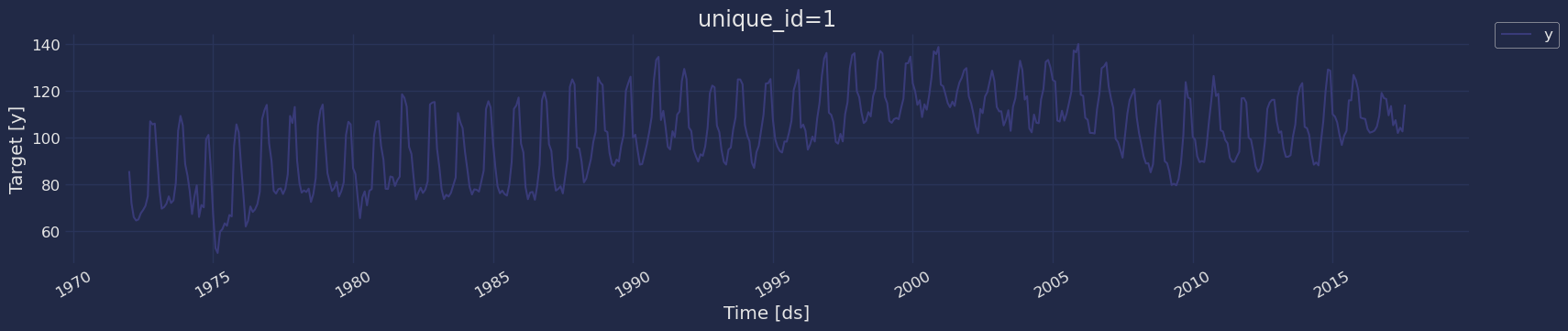
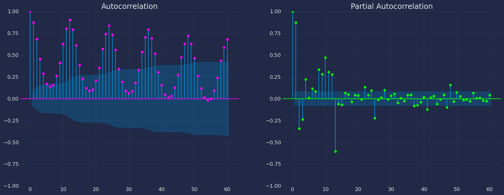
Autocorrelation plots
Split the data into training and testing
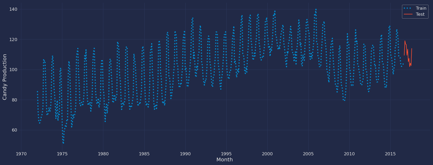
Let’s divide our data into sets 1. Data to train ourAutoTheta model
2. Data to test our model
For the test data we will use the last 12 months to test and evaluate
the performance of our model.
Implementation of AutoTheta with StatsForecast
Load libraries
Instantiate Model
Import and instantiate the models. Setting the argument is sometimes tricky. This article on Seasonal periods by the master, Rob Hyndmann, can be useful.season_length. Automatically selects the best Theta (Standard Theta Model(‘STM’),
Optimized Theta Model (‘OTM’), Dynamic Standard Theta Model
(‘DSTM’), Dynamic Optimized Theta Model (‘DOTM’)) model using mse.
-
freq:a string indicating the frequency of the data. (See panda’s available frequencies.) -
n_jobs:n_jobs: int, number of jobs used in the parallel processing, use -1 for all cores. -
fallback_model:a model to be used if a model fails.
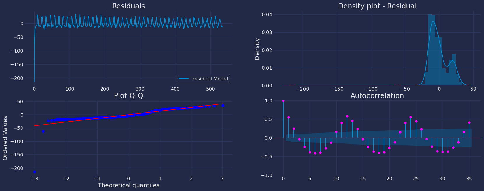
Fit Model
.get() function to extract the element and then we are going to save
it in a pd.DataFrame().
Forecast Method
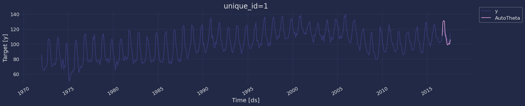
If you want to gain speed in productive settings where you have multiple series or models we recommend using theStatsForecast.forecast method
instead of .fit and .predict.
The main difference is that the .forecast doest not store the fitted
values and is highly scalable in distributed environments.
The forecast method takes two arguments: forecasts next h (horizon)
and level.
-
h (int):represents the forecast h steps into the future. In this case, 12 months ahead. -
level (list of floats):this optional parameter is used for probabilistic forecasting. Set the level (or confidence percentile) of your prediction interval. For example,level=[90]means that the model expects the real value to be inside that interval 90% of the times.
ARIMA and Theta)
Predict method with confidence interval
To generate forecasts use the predict method. The predict method takes two arguments: forecasts the nexth (for
horizon) and level.
-
h (int):represents the forecast h steps into the future. In this case, 12 months ahead. -
level (list of floats):this optional parameter is used for probabilistic forecasting. Set the level (or confidence percentile) of your prediction interval. For example,level=[95]means that the model expects the real value to be inside that interval 95% of the times.

Cross-validation
In previous steps, we’ve taken our historical data to predict the future. However, to asses its accuracy we would also like to know how the model would have performed in the past. To assess the accuracy and robustness of your models on your data perform Cross-Validation. With time series data, Cross Validation is done by defining a sliding window across the historical data and predicting the period following it. This form of cross-validation allows us to arrive at a better estimation of our model’s predictive abilities across a wider range of temporal instances while also keeping the data in the training set contiguous as is required by our models. The following graph depicts such a Cross Validation Strategy: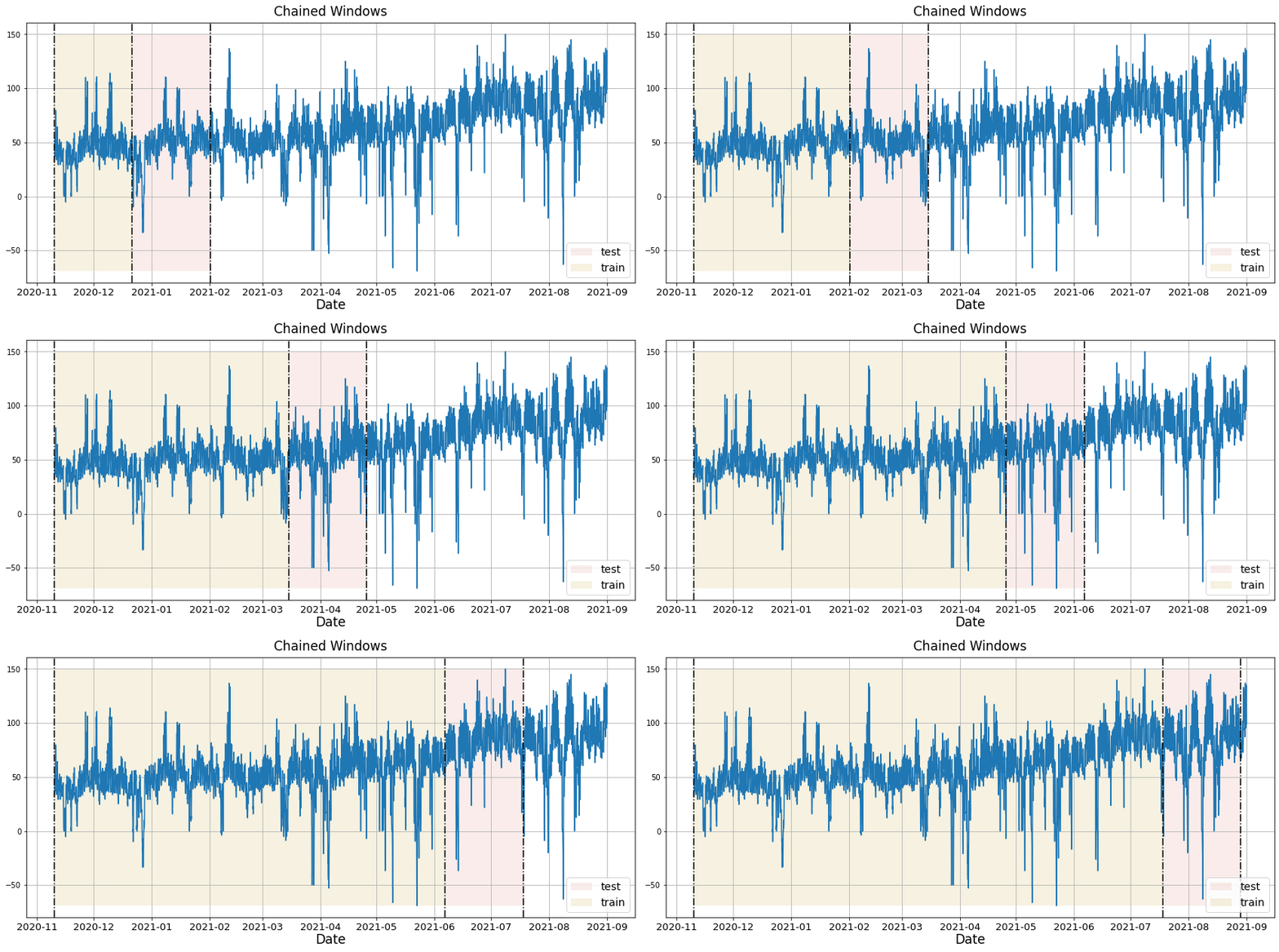
Perform time series cross-validation
Cross-validation of time series models is considered a best practice but most implementations are very slow. The statsforecast library implements cross-validation as a distributed operation, making the process less time-consuming to perform. If you have big datasets you can also perform Cross Validation in a distributed cluster using Ray, Dask or Spark. In this case, we want to evaluate the performance of each model for the last 5 months(n_windows=5), forecasting every second months
(step_size=12). Depending on your computer, this step should take
around 1 min.
The cross_validation method from the StatsForecast class takes the
following arguments.
-
df:training data frame -
h (int):represents h steps into the future that are being forecasted. In this case, 12 months ahead. -
step_size (int):step size between each window. In other words: how often do you want to run the forecasting processes. -
n_windows(int):number of windows used for cross validation. In other words: what number of forecasting processes in the past do you want to evaluate.
unique_id:series identifier.ds:datestamp or temporal indexcutoff:the last datestamp or temporal index for the n_windows.y:true value"model":columns with the model’s name and fitted value.
Model Evaluation
Now we are going to evaluate our model with the results of the predictions, we will use different types of metrics MAE, MAPE, MASE, RMSE, SMAPE to evaluate the accuracy.References
- Jose A. Fiorucci, Tiago R. Pellegrini, Francisco Louzada, Fotios Petropoulos, Anne B. Koehler (2016). “Models for optimising the theta method and their relationship to state space models”. International Journal of Forecasting.
- Nixtla AutoTheta API
- Pandas available frequencies.
- Rob J. Hyndman and George Athanasopoulos (2018). “Forecasting Principles and Practice (3rd ed)”
- Seasonal periods- Rob J Hyndman.